Industry Background
Home health is a nursing specialty in which nurses provide multidimensional home care to patients of all ages. Home health care is a cost efficient way to deliver quality care in the convenience of the client's home.
Home health nurses create care plans to achieve goals based on the client's diagnosis. These plans can include preventive, therapeutic, and rehabilitative actions. Home health nurses also supervise certified nursing assistants. The professional nursing organization for home health nurses is the Home Healthcare Nurses Association (HHNA). Home health care is intended for clients that are well enough to be discharged home, but still require skilled nursing personnel to assess, initiate and oversee nursing interventions.
From Wikipedia: Home Health Nursing
Business Challenge
The primary focus of the home healthcare provider is to keep their patients healthy and out of the hospital. Home healthcare nurses make at-home visits, monitor a patients health, and take measures to proactively address health issues that might require a patient's hospitalization. Beyond individual patient health, there are financial incentives from insurers for home healthcare organization that maintain the patient population under their care healthy and outside of the hospital.
Impact and Outcome
In addition to the BI reports developed for the organization, the hospitalization prediction model provided home healthcare providers with the information needed to focus their attention to patients identified as high-risk when required. Overall, the model was able to differentiate between those patients at risk of hospitalization for particular week vs. those at low risk with about 90% accuracy. For those patients that were flagged at high risk of hospitalization, on average 80% of those patients were correctly identified as requiring hospitalization whereas the remaining 20% were flagged as at risk of hospitalization but were not hospitalized. (The model was tuned with a bias towards identifying high risk patients with the understanding that some patients that were flagged at-risk would not be hospitalized).
2K+
Health statistics and at-home visit history data-points were assessed as inputs to the ML model.
80%
Of true hospitalizations identified among all predicted hospitalizations (i.e., Average recall score for model)
90%
Accuracy for discerning between hospitalizations vs. non-hospitalizations for a particular week (i.e., Average accuracy score for model)
Approach
The following provides an example of the overall approach used for the derivation of the machine learning model. Although every effort was made to maintain the overall relationships and trends reflected in real-world data, the approach presented was developed using synthetic data and is used to highlight the thought-process and methodology used for this type of problem. Below is an outline and links to the sample iPython notebooks used for the analysis.
1. Data Profiling
Data Profiling notebook on GitHub: https://github.com/datastudios/healthcare/blob/master/01_Profile.ipynb
The data was made up of three data sources: patient data, patient visit history, and health statistics captured during those visits:
Patient Data
- There are a total of 1,154 patients
- 673 are female and 481 are male
- The minimum age is 23 and maximum age is 103.
- The average age is ~65 years old.
Visit Data
- The date of the visit
- Total visits to date
- Total hospitalizations to date
- Whether the patient was hospitalized during a particular visit (i.e., visit date)
Health Statistics
- Over 170 health statistic data-points were captured including medications taken, blood pressure, and weight among others.
Imputation Strategy
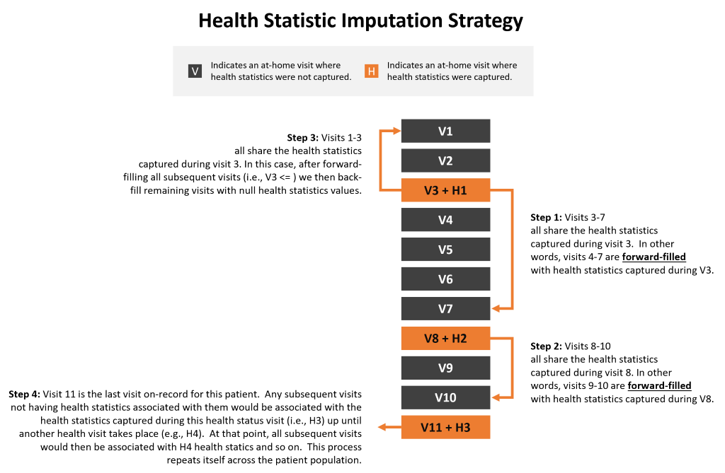
One of the key factors influencing the accuracy of the model's predictions was the imputation strategy for missing data. More specifically, the overall approach for propagating health statistic information captured on some (but not all) at-home health visits would be key. The imputation strategy involved first visits where health statistics were gather and forward-filling those missing values to all subsequent visits up and until there was a more recent set health statistics that had been captured. This ensured that the most recent health data available was associated with visits that came after those statistics were captured. In cases where a visit did not have any health data associated with it after forward-filling, any missing values were then back-filled with the next available health statistic dataset available. And finally, for any patients where a health statistic was never captured (e.g., blood pressure or weight had never been taken) then the mean for the full patient population was imputed. The diagram below provides an overview of this approach:
2. Data Exploration
Data Exploration notebook on GitHub: https://github.com/datastudios/healthcare/blob/master/02_Explore.ipynb
Seasonality
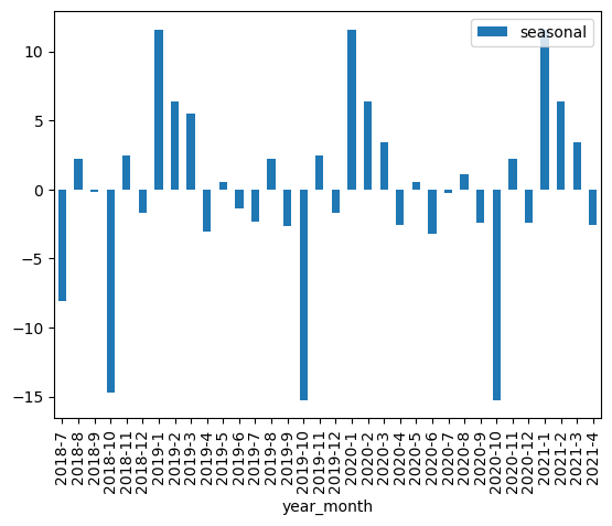
After seasonally decomposing the dataset, it was apparent that their was a clear seasonal component to the data with hospitalizations dropping towards the last quarter of the year and rising sharply at the beginning of each year. This information was used to encode a feature to capture this information.
Distribution
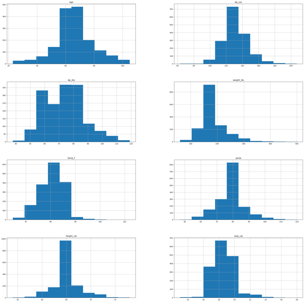
The numeric features of the dataset were for the most part symmetrically distributed with the exception of weight. The weight feature was log transformed to address skewness.
Outliers
Outliers were identified based on the numeric features below. There are a few key indicators of health (e.g., blood pressure readings, weight, and age) where outliers on average reflected higher values than non-outliers.
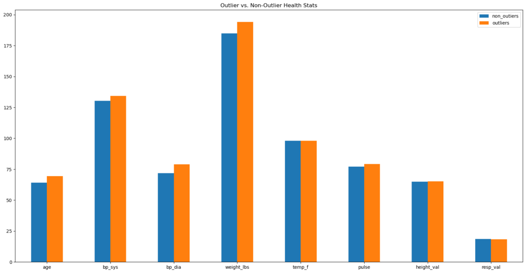
However, it was in the hospitalization per visit ratio that outliers reflected the greatest difference with non-outliers.
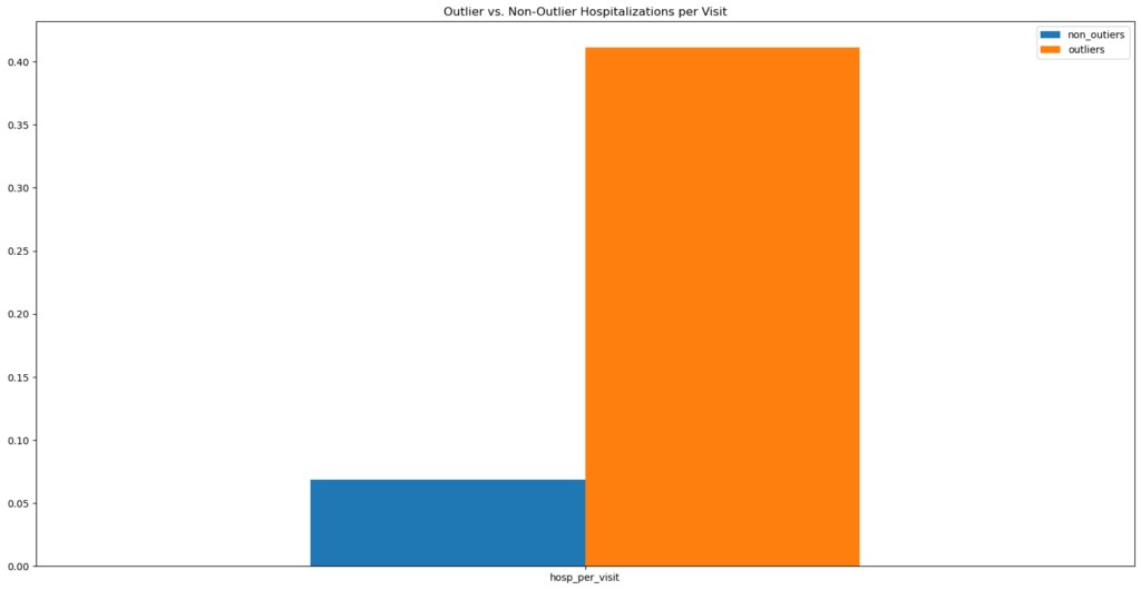
Outliers were not removed from the dataset. However, this information did inform the creation of cluster groups based on the above numeric features to encode this differences.
Cluster Creation
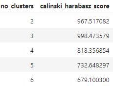
There were 3 clusters identified using the Elbow method and Calinski-Harabasz scores.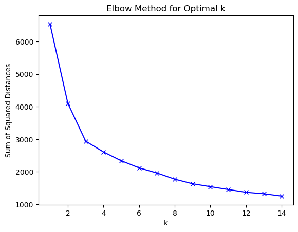
The Calinski Harabasz score confirms 3 clusters being the optimal k.
Lag Variables
Finally, lag variables were created to encode hospitalization and visit history (i.e., hospitalization total, visits total, hospitalization per visit etc.)
3. Prediction
The Prediction and Utilities notebooks bring all the prior profiling and analysis together. The Utilities notebook functions modularize and organizes logic reusable across this and other projects. It also centralizes Scikit-learn custom transformers developed for data transformation and model evaluation steps:
Prediction notebook on GitHub: https://github.com/datastudios/healthcare/blob/master/03_Predict.ipynb
Utilities notebook on GitHub: https://github.com/datastudios/healthcare/blob/master/utils/utils_diagnosis.ipynb
Group Time-Series Cross-Validation
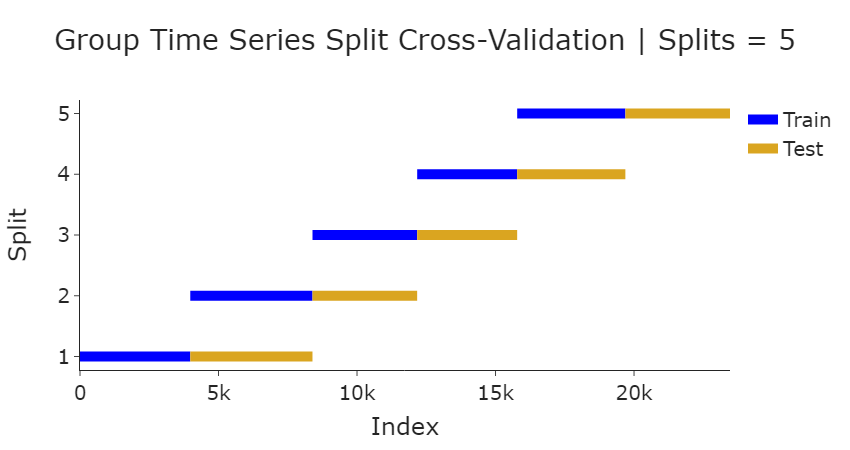
The nature of the dataset requires a time-series based cross-validation approach (a typical random split of the data wouldn't work in this case as it would cause data leakage with future observations "leaking" into training data). Furthermore, the dataset observations may be unevenly grouped since each patient has a different set of visits. So, we'll need to group the train/test splits so that they are split as evenly as possible. The GroupTimeSeries Split API was leveraged as a basis for the custom transformer developed for our pipeline. The diagram below shows the dataset split with the number of splits = 5:
Preprocessor Pipeline
The preprocessor pipeline reflects the functions and custom Scikit-learn classes developed (Step descriptions are purposely verbose, in a production setting these would be kept succinct to allow for experimentation):

Pipeline with Estimator
The full pipeline includes the preprocessing steps along with a custom Scikit-learn RandomizedSearchCV class that instantiates a GroupTimeSeriesSplit object to be used for cross-validation of all models to be tested.

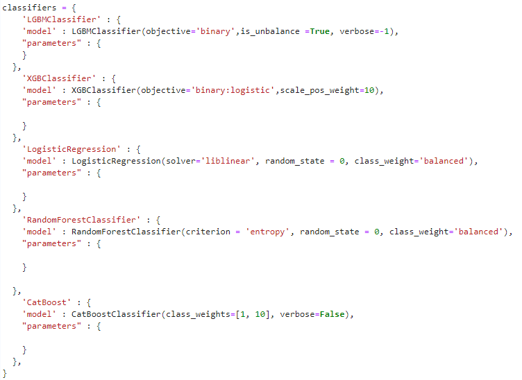
Classifier Dictionary
The classifier dictionary is the data structure containing all models and parameters to be cross-validated. In the example below, we start with baseline parameters. In subsequent steps, we input a distribution of hyperparameters selected for optimization.
Evaluation Function
The evaluation function trains and tests the various models submitted via the classifiers dictionary instantiated previously based on the pipeline steps defined. It returns a data frame containing a summary of results based on the test data submitted and a dictionary containing fitted models along with their predictions.
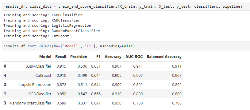
Once the results of the initial set of baseline models is assessed, we can further tune a subset of performant models:
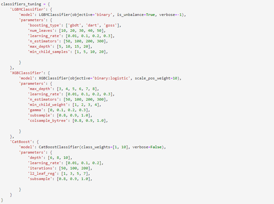
And again obtain result objects as described previously:

Analyze Results
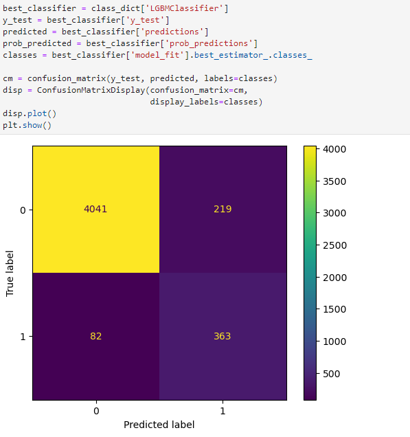
We can then further analyze the results of a candidate model for production. (Here we only show a confusion matrix, but typically we'd want to use a library such as SHAP to better understand and explain the output of the model)
Write Data for BI Tool
Data was then provided for further analysis by business domain experts via their preferred BI tool. (In this example, to CSV files but data was written to the data warehouse for the production version)

Reporting and Analytics
Beyond the model described previously, a full self-service data and analytics environment was enabled for the organization. A sample visualization reflecting model data is provided below:
